How to make a process capability calculation (cp, cpk)?
The process capability cpk, ppk and the machine capability cmk describe the ability to achieve a desired result. In the next minutes, you will use Excel to learn how to calculate machine and process capability. You will be shown the graphs of your values. You could use our online cpk calculator. In addition, you will learn whether your values even meet the requirements for calculating machine and process capability. Further free tools can be found in the toolbox.
This video gives you a quick insight into the Excel template.
Tools for process capability and machine capability analysis (cm)
The desired result of a process is defined by the customer. The customer expects his result to be achieved permanently. The supplier strives to deliver the desired result permanently and at an economically justifiable cost. A supplier achieves this goal by mastering his processes for the provision of services and by establishing and monitoring the corresponding process capability. A process is controlled if the result of the process is predictable. Only a controlled process makes statements about the capability of the process possible.
The customer defines the desired result by a value to be achieved and two specification limits. The limits are called LSL (Lower Specification Limit) and USL (Upper Specification Limit). The limits are also referred to as tolerance limits and thus LTL and UTL.
The tolerance, also called tolerance width, represents the distance between LSL and USL . To evaluate the process capability cpk (process capability index), the requirements of the customer are compared with the results of the process. Here the exceedance share is calculated using a model of the probability of the normal distribution. The exceedance share is the expected number of parts per million that lie outside the limits of the specification.
The objective of the process capability calculation is:
- to obtain an estimate of the proportion of data outside the tolerance limits
- a characterization of the ability of a process to obtain
- obtain an assessment of the possibilities for process improvement
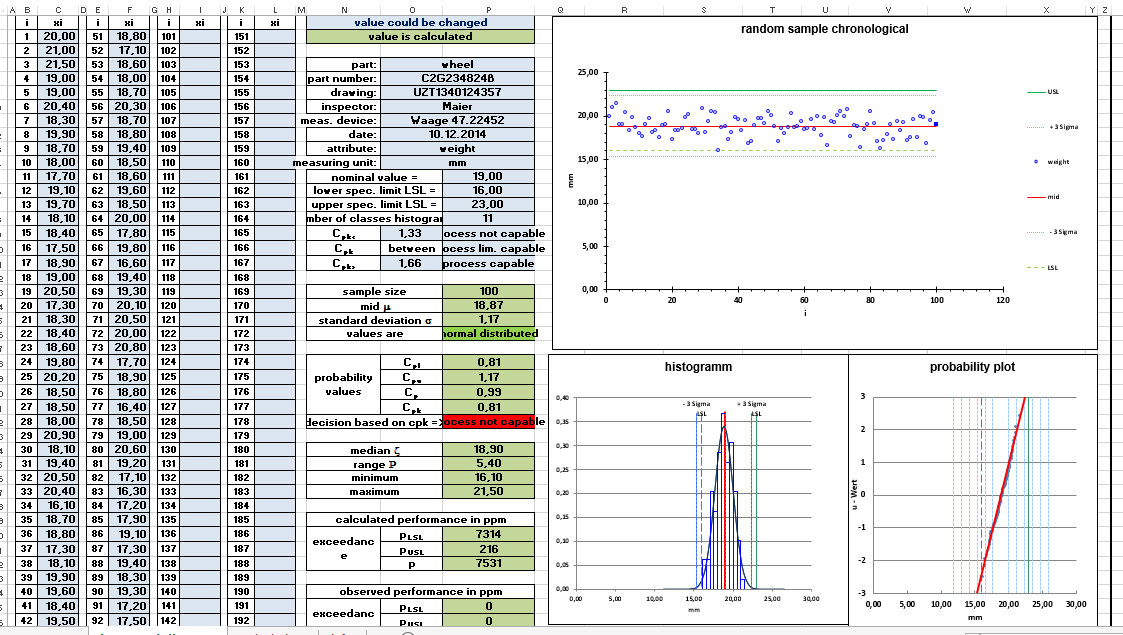
Measurement data is required to calculate the process capability. The measurement data for the comparison of requirement and real process are recorded within the process. The data can be entered into an Excel template for evaluation. The template automatically creates all diagrams and calculates all quality parameters. The normal distribution of the measured values is the basis for the calculation of the data. The statement on the normal distribution can also be found in the Excel file.
If you require proof of machine or process capability using standard software (e.g. Minitab), please send me an e-mail. I will be glad to help you.
| version 1 | version 2 | |
| aim | machine capability | process capability |
| numbers | up to 200 | up to 250 |
| input and calculation | 1 sheet | 1 sheet input 1 sheet output |
| language | german / english / italian | german |
If you want that i make some adjustments for you contact me (if you want to get a template with your company logo or other things).
Feel free to share this post on LinkeIn and other social media.
Excel sheet version 1
You can find a method for the simple and fast transfer of your data from measuring equipment to an excel sheet on the bicsolu.com website.
Capable measuring system as basis for process capability analysis and machine capability analysis
As with all other measurements, the basis for statements about the process is the collection of reliable measurement data. For this it is necessary to qualify the measuring system and its suitability for the measuring task. This is achieved by an MSA (measurement – system – analysis). Detailed contents on measuring system analysis and measuring equipment capability can be found in the article MSA, Measuring System Analysis and Measuring Equipment Capability. The article also contains the corresponding Excel templates For MSA Procedure 1 and MSA Procedure 2.

Statements on process capability and machine capability can be made if the following conditions are fulfilled:
Conditions of process capability
- Variable data must be available (weight, width, length, etc.).
- There must be a sufficient number of measured values available
- The data used must come from a stable process (test for stability).
- The data must follow approximately the normal distribution. (Test for normal distribution)
1. variable data
Data types can be divided into variable data and attributive data. Variable data is data that can be measured. These are for example weight, width, length, thickness etc.. Attributive data is data that cannot be measured as good or bad. No normal distribution can be determined for these data. Statistical key figures can, for example, be percentages (percentage of good parts for the total number of parts).
2. sufficient number of measured values
The absolute lower limit for investigating a value for the capability of a process is 50 values. The results of the meaningfulness at 50 values, however, are afflicted with a certain vagueness. 50 values are the number of measured values for the short-term capability examination or also machine capability examination.
A minimum of 100 parts applies to the preliminary process capability test. For the long-term investigation of process capability, the recommendations are shown in the overview „Process capability over time“.
The definition of the sufficient number of measured values is based on VDA Volume 4 Part 1 and DGQ.
3. process stability
A process can be influenced by ordinary and extraordinary causes. Ordinary causes are caused by the natural process dispersion that is present in every process. Exceptional causes are causes that are not considered a normal part of the process. They are caused by one-time or recurring actions and events. Examples are changes in machine settings, systematic changes in raw materials, etc.
The first step is to discover, eliminate or control these extraordinary events in the process. The basis for the separation of ordinary from extraordinary causes is an understanding of the process to be investigated. As long as the systematic causes are not under control, a process capability analysis makes no sense. If the systematic causes are under control, the dispersion in the process is reduced to the usual causes.
A process is stable if it is not scattered by unusual causes. In process monitoring, process diagrams or control charts are used to represent process stability or to document exceptional values. The process diagrams or control charts are generally examined for the 4 most important exceptional conditions:
1 point more than 3S from the centerline -> Indication of a displacement of the mean, standard deviation or a single outlier in measurement
9 successive points on one side of the centerline -> Indication of a shift of the mean value
6 consecutive points all increasing or decreasing -> signs of a trend
14 consecutive points, alternating up and down -> signs that the data comes from two different sources
If none of these exception conditions is met, the process is considered stable. The first condition for calculating the process capability is fulfilled.
I have created an Excel template that tests the 8 rules of stability. You can find the corresponding article here.
4. normal distribution
The distribution of the measured values can be displayed in the histogram. In the histogram, the data is supplemented with data on the normal distribution so that both representations can be compared. This is a rough view. A more exact statement on normal distribution can be made by corresponding calculations. An additional graphical option for displaying the normal distribution is offered by the probability mesh. The diagram data is transformed into a probability network. A diagram is generated by transforming the data. If the diagram data are close to the idealized straight line, a normal distribution can be assumed.
Histogram and probability net can be found in the Excel template. By checking the data for normal distribution, the second prerequisite for calculating the process capability is fulfilled in addition to the confirmed process stability. The Excel template takes care of the graphical examination of the normal distribution for you. The Excel template for the mathematical test for normal distribution can be found in the article „Test for Normal Distribution Anderson Darling“. The tests for normal distribution have different properties with regard to the type of deviations from the normal distribution that they detect. The Anderson Darling Test has proven to be a reliable test for normal distribution. Therefore, I carry out the mathematical test for normal distribution with the Anderson Darling Test. The test is also used in the template for machine and process capability.
Capability metrics for non-normally distributed characteristics
It can happen that characteristics are not – normally distributed. This applies in particular to the characteristics:
- flatness
- roundness
- parallelism
- perpendicularity
- etc.
These characteristics are characterized by the fact that the characteristics are often limited by a 0 value. If you need assistance with the evaluation of such characteristics in the context of the investigation of process capabilities, please write to me at (roland.schnurr@sixsigmablackbelt.de).
The Process key figures sorted by process phase
The capability and controllability of a process is determined on the basis of quality indicators, which result from mean value, tolerance limits and dispersion.
The subdivision and definition of the individual indicators is based on the guidelines of the VDA (Verband der Automobilindustrie e.V.) and the DGQ (Deutsche Gesellschaft für Qualität).
If one considers the temporal course of process capability, it is generally divided into 2 groups:
- Process capability before series start subdivided into
- Short-term capability of a process or machine
- Provisional process capability
- Process capability after start of production synonymous with long-term process capability
Machine capability or short-term capability of a process
In practice, it can often happen that not enough parts are available to determine the provisional process capability. If this is the case, an analysis of the machine capability or short-term capability of the process is carried out. This is often the case with preliminary inspections of production equipment at the manufacturer’s or during the running-in of production processes.
In the mfu machine capability test, all parameters (human, method, material and environment) are kept constant so that, if possible, only the influence of the machine on the result can be measured. This means there is:
- no change of machine operators
- no change in the operation of the machine
- no change to the material batch
- environment parameters as constant as possible
- etc.
Influences which cannot be avoided and which are not accidental are documented. These influences are then separated and sorted.
A preliminary statement about the suitability of the process is determined. The characteristic number for the machine capability is the cmk value. The cmk value results from the minimum of cmu and cmo.
Normally 50 consecutive parts are taken from the process. The chronological sequence of the parts is documented in order to identify possible trends. The 50 parts are also used to check the distribution form of the measurement results.
Provisional process capability
The preliminary process capability analysis is used to examine a process before the start of series production. At the same time, it helps to declare the upper and lower intervention limits of the process. Methodology: The process is run over a longer period of time. During processing, random samples are taken at regular intervals. As a guideline, 25 samples are taken, each with five parts. The minimum is 20 samples with three parts each.
A quality control chart is used to assess whether the process is controlled. At the same time, the measured values can be evaluated via additional analyses. This is helpful here:
Already in this phase of the analysis the process should produce under the future series conditions. All influences of the series should already be present and effective. At the same time, the methods and formulas for calculating the individual capability figures should already be used in determining the short-term capability and in calculating the machine capability. This is the only way to ensure a meaningful link between the individual analyses over time.
Long-term process capability
The long-term process capability index cpk defines the results of the process after the start of series production. Methodology: The long-term process capability analysis is intended to assess the quality capability under real conditions. It therefore extends over a longer period of time. Ideally, random samples are taken over 20 days of production. The procedure corresponds to the analysis for short-term process capability.
Short-term and long-term process capability investigations analyse the manufacturing process with regard to its suitability to fulfil the planned manufacturing task within the specified quality requirements. In the long-term process capability analysis, the individual influences of the 5 types of influence also become much more apparent than in the short-term analysis.
The formula for calculating the individual key figures does not change with respect to time. The formulas for Cm = Pp = Cp are independent of the time. Only the scope of the measured values changes. The same procedure applies to the formulas for Cmk = Ppk = Cpk.
As an example, I will explain the calculation of the key figures on the basis of the long-term process capability.
The long-term process capability is described by the cp value (process capability) and the cpk value (critical process capability). The parameters are determined according to the following formulas.
CP = process dispersion
CPO = process variation upper tolerance limit
CPU = process variation lower tolerance limit
CPK = process variation and position
OTG = Upper tolerance limit
UTG = lower tolerance limit
x transverse = mean value
s = standard deviation
CP value
The Cp value describes the process potential. The key figure cp is a measure of the width of the process variance in relation to the tolerance width. The tolerance width is the range between the upper and lower limit value. The width of the process variance is usually three times the standard deviation upwards or downwards around the mean value. Within this range, more than 99% of all values are expected for a controlled process.
The cp value is 1 if the process deviation range corresponds to the tolerance limit (upper/lower limit value). The calculation of the cp value is not sufficient for assessing the quality capability of a process, since it does not take into account the position of the process. The cpk value is used for this purpose.
Process capability index CPK Value
The cpk value (process capability value) is equal to the process potential cp, but also takes into account the position of the distribution by calculating the critical distance between the process position and the tolerance limit. The process capability index cpk value is defined so that it is equal to the cp value if the process is centered in the tolerance center. The cpk value corresponds to the smaller or more critical value of cpo or cpu. If the cpk value is smaller than the cp value, this means that the mean value of the distribution is outside the tolerance center. If cp is greater than the process capability index cpk , the process can be made capable by centring.
If you want to know which values mean value and standard deviation must fulfill in order to reach a target value cp or a target value cpk, you can use the Excel template from the article „Calculate cp and cpk“.
An examination of the ability may only be carried out in the case of controlled processes. The process capability index cpk is a measure for the characteristic position and scatter of the characteristics. The position and scatter contains influencing factors which are triggered by the 5 M, man, machine, method, material and environment. The cpk value is therefore a good measure to analyze the effects of different influencing factors, is the Ishikawa or cause – effect – diagram.
Cpk and scrap correlation in % and ppm
The capability indices cp and cpk are used for process control. They enable statistical process control through the combination of mean value and standard deviation. The capability indices are compared with the customer’s requirements, thus enabling a prediction of the process’s capability.
If the capability of a process cannot be proven, no statements about the correctness of the output are possible. If it is not possible to make statements about the absence of errors in advance and only good output results are to be passed on, a 100% check of the results is unavoidable.
If a control of the results is only possible via a destructive test, the complete output would have to be tested destructively, since 100 % control would be destroyed. The basis for random testing is often the machine or process capability.
If a cpk can be calculated, then predictions can be made to the reject of the process. Assuming a normal distribution, the following scrap results for the following cpk values in percent or in parts per million.
| Number of Sigma up to the tolerance limits | cpk – value | scrap in % | scrap in ppm |
| 1 | 0,33 | 32 % | 320000 |
| 2 | 0,67 | 4,60 % | 46000 |
| 3 | 1,00 | 0,27 % | 2700 |
| 4 | 1,33 | 0,0063 % | 63 |
| 5 | 1,67 | 0,000057 % | 0,57 |
| 6 | 2,00 | 0,0000002 % | 0,0002 |
Process capability with one-sided tolerance
If a characteristic on a page has a specification limit, you cannot specify a tolerance width. Therefore, only the Cpk value (process capability value) can be calculated for one-sided tolerance.
If an upper specification limit is specified, the process capability index corresponds to Cpk = Cpko. If a lower specification limit is specified, the Cpk = Cpku corresponds.
Process capability and machine capability with Minitab or R software
Minitab is the default package in the Statistics section. You can download the free 30 day version here.
Process capability and machine capability with the statistics software R
If you do not have the possibility to use Excel, we recommend the free statistic software R as an alternative.
For the data of the Excel template from above, I now use R as statistics software for the evaluations.
After you have installed R, install the extension package qualitytools. After appropriate preparation of the data you receive the following evaluation by the execution of the command cp.
# Import data from Excel file maschinen.xlsx into table df1
# Then call the cp function from the library qualitytools
library(openxlsx)
library(qualityTools)
xlsxFile <- („C://Users//ThinkPad User//Data//R Statistics// Machines.xlsx“)
df1 <- read.xlsx(xlsxFile = xlsxFile, sheet = 1, startRow = 1, skipEmptyRows = FALSE)
cp(df1$mm,,23,16)
Plot time series with the statistics software R
The package ggplot2 must be installed and activated. Then we start creating the time series diagram.
# Data is already in table df1
# define the data area
# Packet ggplot2 is initialized
library(ggplot2)
# Calculate the number of values in the value range
NumberValue <- length(df1$mm)
x<-(1:NumberValue)
# define the data area
g<-ggplot(df1, aes(x,df1$mm))
# define the data points
g<- g + geom_point()
g<- g + geom_point(colour=“blue“, size= 2)
# define the connecting line between the data points
g<- g + geom_line(colour= „black“)
# define the upper limit as a line
g<- g + geom_hline(yintercept=23 ,colour= „darkgreen“, size = 1 )
# define the lower limit as a line
g<- g + geom_hline(yintercept=16 ,colour= „darkgreen“, size = 1 )
# calculate the mean value and enter it in the diagram
Average <- mean(df1$mm)
g<- g + geom_hline(yintercept= mean value ,colour= „red“, size = 1 )
You see the following graphic
Meanwhile I often use the statistics software R to compare the results from Excel. I find R quite useful, although it takes some time to get used to it.